SVETLANA PANASYUK
Medical Hyperspectral Imaging
Optical Metrology
Tissue Spectroscopy
Mantle Flow
GPS
Remote Sensing
Image Processing
Fun
Reference Earth Model
|
There are a few more tricky questions, of course, which we discuss and analyze in
the GJR paper. If you follow the next two links, you can download
spherical harmonic expansions (up to l,m=25) for our model of dynamic
topography and corresponding geoid. Here I present pictures from the paper hoping that I can share the excitement of these new results with you! 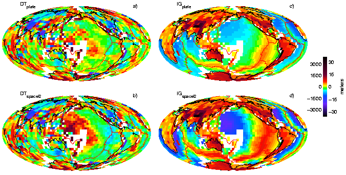
Picture above shows four fields on a 5-by-5 degree grid: two for topography (a and b), and two for geoid (c and d). The topography is the total isobaric surface topography calculated from ETOPO5 topography that was corrected for the topography due to isostatically compensated crust, oceanic lithosphere (two models), and tectosphere. The oceanic lithosphere is modeled as plate cooling (a) and as half-space cooling (b). The geoid fields are the total geoid due to isostatically compensated crust, oceanic lithosphere (two models), and tectosphere; the oceanic lithosphere is modeled as plate cooling (c) and as half-space cooling (d). White areas have no data coverage. The dynamic topography fields displayed above show large variations over adjacent grid-cells, which are very unlikely to be supported by the large-scale convective flow. Those short-wavelength variations are probably due to the errors/uncertainties in the models we used. Each component of the total field (contributions from crust, lithosphere, and tectosphere) has uncertainties associated with the data and assumptions used to build each model. Some areas do not have data coverage at all (e.g., West Pacific plateaus and the Arctic do not have reliable ocean floor age data). To gain robustness in our model, we estimate the errors in dynamic topography at every grid point. In a similar way, we calculate the errors related to the residual (observed minus isostatic) geoid anomaly, assuming that the horizontal scales of the dynamic topography and the geoid anomaly are similar. The picture below shows the uncertainties in the dynamic topography (e) and geoid (f), when the oceanic lithosphere is modeled as plate cooling. The color bar for uncertainties in dynamic topography and geoid is clipped at 1600 m and 40 m, correspondingly. White areas have no data coverage. 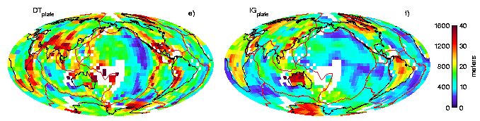
|
 Isostatic Topography and Geoid
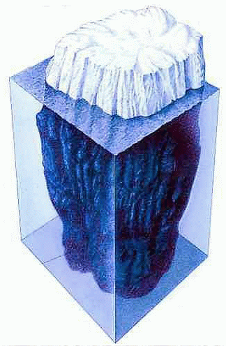 have been
recognized quite a long time ago: beginning of the last century? Then, scientists suggested that what we see on the
Earth surface is actually only "upper part of an iceberg" - the main structure is hidden below the sea level.
In another words: the crust is in an isostatic equilibrium. As an iceberg, the long-lived crustal formations are
mainly submerged into the upper mantle.
Since the ice is much heavier than air and lighter than water (the whole atmosphere above you weights
as much as 10 meters of water, or only 3 meters of rocks below your feet!), the height of what sticks out in the
air is much less of what is hidden below.
have been
recognized quite a long time ago: beginning of the last century? Then, scientists suggested that what we see on the
Earth surface is actually only "upper part of an iceberg" - the main structure is hidden below the sea level.
In another words: the crust is in an isostatic equilibrium. As an iceberg, the long-lived crustal formations are
mainly submerged into the upper mantle.
Since the ice is much heavier than air and lighter than water (the whole atmosphere above you weights
as much as 10 meters of water, or only 3 meters of rocks below your feet!), the height of what sticks out in the
air is much less of what is hidden below.