Inversion for mantle structure is a very non-unique problem. In simple words the problem can be stated as following (see diagram below).

We can observe/measure several fields: equipotential surface (dV) of gravity field, plate velocity on the Earth surface (v), topography of the Earth surface (da) and the Core-Mantle boundary (dc). These are the "Reality".

We can estimate the seismic velocity anomalies inside the Earth mantle, profiles of gravitational acceleration and density. These are the "Data".

Then, we can convert the seismic anomaly into density anomaly and consider it as a driving mechanism of the mantle flow.

Thus, we build a model of convecting Earth mantle. The model allows us to calculate geoid, plate velocity, topography, etc. These physical fields we compare with the "Reality", the real geoid, velocity, and topography.

By varying the model parameters, e.g. viscosity structure and/or density variations, we try to fit the observables as much as possible. Since the model has many parameters, and our understanding of Earth physics is still incomplete, the problem produces many solutions which we try to reduce to the ones close to a reality. I started working on mantle properties inversion at MIT. The research grew into a few chapters of my Doctoral thesis. My paper, "Inversion for Mantle Viscosity Profiles Constrained by Dynamic Topography and the Geoid, and Their Estimated Errors", came out later in GJI, which I worked on in collaboration with my thesis advisor, Brad Hager. 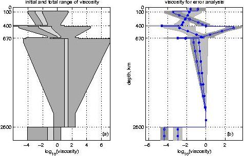If you would like to know more, read a short summary of the paper below, or look up the paper and its abstract.

SUMMARY
We perform a joint inversion of Earth's geoid and dynamic topography for radial mantle viscosity structure using a number of models of interior density heterogeneities, including an assessment of the error budget. We identify three classes of errors; those related to the density perturbations used as input, those due to insufficiently constrained observables, and those due to the limitations of our analytical model.

We estimate the amplitudes of these errors in the spectral domain. Our minimization function weights the squared deviations of the compared quantities with the corresponding errors, so that the components with more reliability contribute to the solution more strongly than less certain ones. We develop a quasi-analytical solution for mantle flow in a compressible, spherical shell with Newtonian rheology, allowing for continuous radial variations of viscosity, together with a possible reduction of viscosity within the phase change regions due to the effects of transformational superplasticity.

The inversion reveals three distinct families of viscosity profiles, all of which have an order of magnitude stiffening within the lower mantle, followed by a soft D"-layer. The main distinction among the families is the location of the lowest-viscosity region, -- directly beneath the lithosphere, just above 400-km, or just above 670-km depth. All profiles have a reduction of viscosity within one or more of the major phase transformations, leading to reduced dynamic topography, so that whole-mantle convection is consistent with small surface topography.

Decimal logarithm of relative mantle viscosity versus depth (km). a) Inversions are started from a randomly chosen viscosity profile constrained by the light gray shading. During the inversions, the viscosity is allowed to vary within the dark gray shading area. 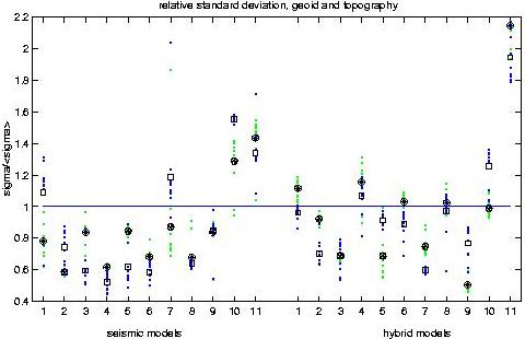b) The logarithmic mean of 11 viscosity profiles for each density anomaly group chosen for the first-step of the error analysis (solid line with the squares centered at each step corresponds to the hybrid models group, solid line with the circles – to the pure seismic models group) and the standard deviation around the mean (dark and light gray shading is for hybrid and pure-seismic groups, correspondingly).

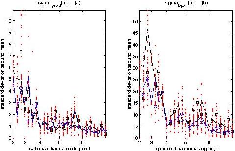
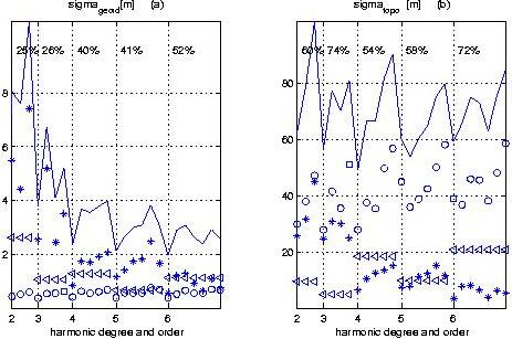
Geoid (light dots) and topography (dark dots) standard deviations for each viscosity profile (total of 11 as in the figure above) and each density model (abscissa) normalized by the mean within each group. The std averaged over the viscosity profiles is shown by wheels (geoid) and squares (topography) for each density model.

Uncertainty in the density anomaly models, geoid (a) and topography (b) in meters, versus spherical harmonic degree and order. The dots are the standard deviations for each viscosity profile (from assemblages as in first figure). The solid lines connect cosine spherical harmonic coefficients that are averaged over the viscosity profiles (dark line is for the hybrid group and light line is for pure-seismic group). The symbols correspond to non-zero sine spherical harmonic coefficients (squares for hybrid group and circles for pure-seismic group).

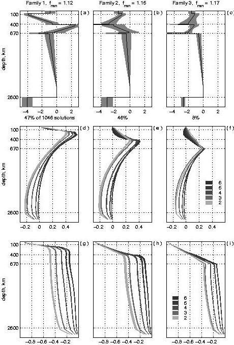
The total error rms (solid line), geoid (a) and topography (b) in meters, versus spherical harmonic degree and order. Three types of errors are show: the density model uncertainty (asterisks), the observational error (circles), and the modeling errors (triangles). The numbers on the top show the percent of the harmonic degree error relative to the total signal amplitude of the same harmonic.

Results of the inversion form three families, shown in columns one, two, and three. The decimal logarithm of relative mantle viscosity for each family is shown versus depth (km) for the first (a), second (b), and third (c) family, with the weighted average (solid line), the standard deviation (shaded area), and the weighted minimization function Fmin. Geoid kernels for spherical harmonics l=2-6 corresponding to the three families of mantle viscosity profiles are shown in (d-f). Surface dynamic topography kernels for spherical harmonics l=2-6 corresponding to the three families of mantle viscosity profiles are shown in (g-i). 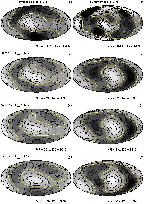(For clarity, only one fifth of the standard deviation around the weighted average is shown in Figs (d-i).

The dynamic geoid (left column) and the dynamic topography (right column). The estimated fields are shown in (a) and (b) and saturated in color. The means within each solution-family are plotted in (c) and (d), (e) and (f), (g) and (h) for the first, second, and third families, respectively. The contour levels are 20 m (geoid) and 100 m (topography), zero level is white, and positive values are lighter. 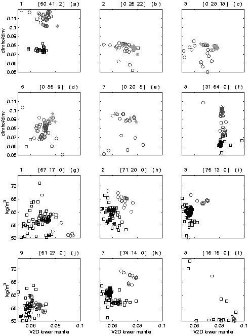The fitting criteria, fmin, the variance reduction, VR, and the degree correlation, DC, are shown for each family solution.

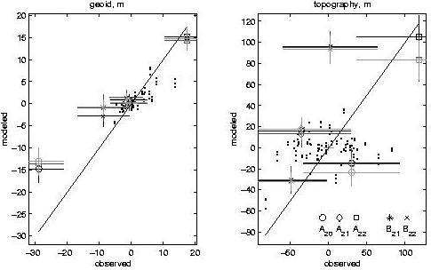
The conversion factor determined for the density models. The abscissa corresponds to the dlnr/dlnv-value of the lower mantle. The ordinate is the dlnr/dlnv-value of the upper mantle for pure-seismic models (a-f), and the slab density contrast (kg m-3) relative to the ambient mantle density for the hybrid-models (g-l). Solutions correspond to the first, second and third viscosity families (squares, circles, and asterisks, respectively)

The spherical harmonic coefficients (l=2-6) of the modeled fields, geoid (a) and topography (b), versus those of the observed fields. The dots correspond to coefficients (l=3-6), whereas markers denote l=2 components according to the legend. The mean of the first family solutions is shown by black, of the second by dark gray, and of the third by light gray. The error bars represent uncertainties of the observed fields versus std of the modeled field coefficients within each solution family. The diagonal line represents a perfect fit.